Help

Define your experimental data in this section. More then one file can be uploaded, each file representing data measured at different magnetic field. If data were measured at multiple field strengths, the residue types and numbers will be compared and chemical shift differences fitted globally to calculate kinetic parameters.

The input-file should have the following format:

1st line	Value of the B0 field for the nuclei of interest in MHz (e.g. 60.12).
2nd line	Value of the constant relaxation time for the CPMG experiment in seconds (e.g. 0.04).
3rd line	Comment line. In the example file, we described the data format (e.g. #nu_cpmg(Hz) R2(1/s) Esd(R2)).
> 3rd line	The first line of the block defines the residue type and number and optionally the intrinsic relaxation rate R20 from HEROINE experiment. The following lines contain the CPMG frequencies (, s-1), relaxation rates (, s-1) and errors in relaxation rates (, s-1).

60.12
0.040000
#nu_cpmg(Hz)        R2(1/s)      Esd(R2)
# A1
  50.000   37.060    0.746
 100.000   38.590    0.738
 200.000   37.794    0.725
 300.000   34.686    0.700
 400.000   32.837    0.639
 500.000   27.971    0.583
 600.000   27.488    0.541
 700.000   26.366    0.510
 800.000   23.926    0.488
 900.000   23.141    0.472
1000.000   22.697    0.459
# B2
  50.000   32.844    0.656
 100.000   32.088    0.639
 200.000   30.126    0.593
...
  

60.12
0.040000
#nu_cpmg(Hz)        R2(1/s)      Esd(R2)
# A1   R2_0:   20.000
  50.000   37.060    0.746
 100.000   38.590    0.738
 200.000   37.794    0.725
 300.000   34.686    0.700
 400.000   32.837    0.639
 500.000   27.971    0.583
 600.000   27.488    0.541
 700.000   26.366    0.510
 800.000   23.926    0.488
 900.000   23.141    0.472
1000.000   22.697    0.459
# B2   R2_0:   20.000
  50.000   32.844    0.656
 100.000   32.088    0.639
 200.000   30.126    0.593
...
  

In this section, the user selects an appropriate set of residues. ShereKhan's suggestion is based on the calculation of the α-values. If data at several B₀ fields are provided, ShereKhan performs the following analysis of the exchange regimes [5]:

where

B0, high/low are the field strength values for the highest and lowest fields defined, and Rex, high/low are the exchange terms for the highest and lowest fields defined.

The calculated α-values can be used to estimate the exchange regime:

In this section, the user can select a model for fitting the data based on a chosen exchange regime.

The fittings presume the following kinetic scheme:

The following formulas are used to calculate R_2,eff for different models such as the Bloch-McConnell [1], Carver-Richards [2, 3] and Luz-Meiboom [4] models:

Bloch-McConnell model
Carver-Richards model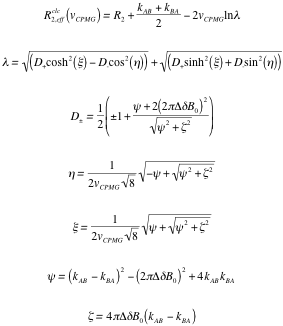
Luz-Meiboom model

where

TCP given constant relaxation delay given CPMG frequency B0 given field strength for the nuclei of the interest in MHz R2 fitted intrinsic transverse relaxation rate kAB, kBA fitted kinetic rate constants (slow exchange) kex fitted kinetic rate constant (fast exchange) Δδ fitted chemical shift difference in ppm (slow exchange) φ fitted population weighted chemical shift difference in ppm2 (fast exchange)

The optimization of the parameters is performed by minimizing the target function:

where

given experimental relaxation rate given experimental error in the relaxation rate calculated relaxation rate based on model

The kinetic rate constants k_AB and k_BA and the chemical shift differences Δδ are grid-searched for the determination of the starting parameters, globally and locally, respectively. User can access the details of the grid search in the advanced options tab.

The results of the calculations are presented in this section. The values of globally fitted parameters are:

Slow exchange	Forward and backward rates kAB and kBA Exchange rate kex = kAB + kBA Population
Fast exchange	Exchange rate kex = kAB + kBA

The chemical shift differences Δδ for the slow exchange regime and population weighted chemical shift differences φ for the fast exchange regime are fitted separately for each residue. Intrinsic relaxation rates are fitted for each residue and each B₀ field value.

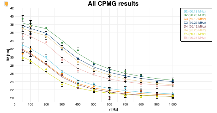
ShereKhan provides a graphical presentation of the experimental and calculated dispersion profiles. Moreover, plots for individual residues are available to check the details of the fitting results. Additional plots either shows chemical shift differences Δδ for the slow exchange regime or φ values for the fast exchange regime. A pdf file with dispersion curves and a summary output file (log file) are available for download.

Graphics

Fitting of the experimental data. The graphs can be downloaded in SVG, PDF, PNG and JPG format. Moving over the residues in the legend (top right corner) will highlight the corresponding data of the respective amino acid at the given field strength.

[1]	McConnell, H. M. (1958) Reaction rates by nuclear magnetic resonance, J. Chem. Phys. 28, 430- 431
[2]	Davis, D.G. et al. (1994) Direct measurements of the dissociation-rate constant for inhibitor-enzyme complexes via the T1 rho and T2 (CPMG) methods. J. Magn. Reson. B, 104, 266–275.
[3]	Carver, J. P.; Richards, R. E. (1972) General 2-site solution for chemical exchange produced dependence of T2 upon Carr-Purcell pulse separation J. Magn. Reson., 6, 89-96.
[4]	Luz, Z. and Meiboom, S. (1963) Nuclear Magnetic Resonance study of the protolysis of trimethylammonium ion in aqueous solution—order of the reaction with respect to solvent. J. Chem. Phys., 39, 366–370.
[5]	Millet, O. et al. (2000) The static magnetic field dependence of chemical exchange linebroadening defines the NMR chemical shift time scale. J. Am. Chem. Soc., 122, 2867–2877.